Where Neural Networks Earn Their Keep in Demand Planning
Demand curves bend in ways a straight line can't follow, and punish anyone who chases every wiggle in the data. Here's how we decide when a neural network belongs in the forecast, how we build one that survives a 150-week history, and why it never runs alone.
Why nonlinearity is the story
For most of demand planning's history, "model" meant a formula you could write on a whiteboard: a moving average, a seasonal index, an exponentially weighted trend. Those models are still the right choice for most of a typical catalog: they're stable, explainable, and cheap to compute across tens of thousands of product-and-market combinations (we call them combos) every week. The trouble starts at the combos where demand doesn't move in a straight line no matter how you transform it.
Price elasticity isn't constant; it often steepens sharply past a specific discount threshold. A promotion's lift depends on how recently the item was promoted before it, not just on the promotion itself. Weather affects a beverage combo only once temperature crosses a point shoppers actually notice. Every one of these is an interaction effect (the impact of one variable changes depending on the value of another).
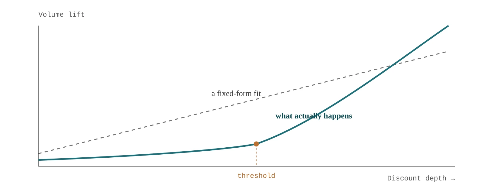
A well-built regression can capture a good deal of this. Transformed drivers let its response curve bend, and statistical testing can decide automatically which candidate terms earn a place. But it can only test the shapes and combinations it's been offered. A neural network works without that menu. Given enough signal-bearing history, it can find that price matters only in combination with promotion depth, or that trend and day-of-week compound near a holiday, or locate a threshold nobody knew to look for, and learn the shape of that interaction directly from the data.
Neural networks aren't the only models that can do this. Tree-based methods, such as gradient-boosted trees, also find interactions on their own and are a serious contender on tabular data like this. Which kind wins depends on the product, the driver set, and how much history exists, which is why no model here gets to run alone (more on that in section 5).
A regression captures curvature through the transformations and candidate terms it's given. A network can find a bend like this one, where a driver's effect barely registers and then rises sharply, including where it sits, without its form being specified in advance.
What the network actually learns from
A neural network is only as good as what you hand it, and in demand planning what you hand it is a regressor library: the same driver variables that feed every other model in the lineup. Price, promotional volume, trend, out-of-stock percentage, point-of-sale volume, a customer-provided forecast where one exists, external variables like weather or an economic index, and calendar effects (day-of-week, month-of-year, holiday proximity). Each product and market combination assembles its own regressor set from whichever of these actually apply to it. For how these drivers fit into the wider forecasting approach, see Intelligent Forecasting with AI.
Two housekeeping details matter more than the architecture itself. First, every column is normalized (centered and scaled) before it reaches the network, because price measured in dollars and promotional volume measured in units live on wildly different scales, and an un-normalized input dominates the gradient by accident of unit rather than by actual importance. Second, whatever the model predicts has to be converted back into real volume before a planner sees it, because a forecast left in standardized units is a number nobody can read.
The activation function is what lets a network bend instead of drawing straight lines, and different curves suit different kinds of response. A logistic curve suits a response that levels off. A rectified linear unit, or ReLU, suits an effect that stays off until a threshold and then rises steadily. A hyperbolic tangent or soft-sign curve suits a relationship that can push volume up or down around a center point.
Training small models well, not big models once
In plain terms: With only about 150 weeks of data per product, a network can easily memorize the past instead of learning from it. The settings below exist to prevent that: small noisy updates, smoothing, a separate step size for each input, and a penalty on complexity. If you just want the takeaway, skip ahead to section 4.
Here's the detail that separates demand planning from most of the world neural networks were built for: a typical product's usable history is two or three years of weekly data, on the order of 150 points. That is tiny. It means the training procedure matters more than the network's size, because a network with enough free parameters can memorize 150 points instead of learning from them, and a memorized network looks perfect on history and then fails on the next quarter.
So the network trains in small mini-batches rather than on the full history at once, which adds a little noise to every update and makes it harder for the model to lock onto any one stretch of weeks. A momentum term smooths that noise across updates. And instead of one global learning rate, each weight gets its own step size, scaled by the size of its recent gradients, the error signals that tell each weight which way to move. A weight whose gradients have been consistently large gets damped, and one whose gradients have been small gets a relative boost. The effect is that a loud input, like a promotional flag that flips on and off, doesn't dominate training just because its signal is bigger.
Core training parameters, tuned per model rather than left at framework defaults
Symbol
Role
Why it's there
η
Learning rate
Base step size for each weight update, rescaled per-parameter by accumulated gradient history
μ
Momentum
Carries a fraction of the previous update forward, smoothing week-to-week gradient noise
λ
Regularization
Discourages weights from growing large enough to memorize a short history
α
Decay
Controls how quickly the per-weight gradient average forgets older batches
None of this is exotic. It's the standard toolkit for training on scarce data: mini-batching, momentum, adaptive per-parameter rates, and an explicit penalty on model complexity. What's specific to demand planning is applying that toolkit at a scale most neural network training was never designed for, and re-tuning it automatically rather than by hand.
Giving demand a memory
A feedforward network treats every week as independent once its regressor values are computed. That's a real limitation for demand that carries momentum from one week into the next: the dip that follows a promotion, the ramp-up after a stockout clears, a trend that's still accelerating. Where recent trajectory predicts the next few weeks better than any single driver can, a model needs some way to remember it: an internal state that carries forward from one week to the next, updated rather than recomputed at every step, so it can weigh what's new against what it already believed.
That's the same basic idea behind the recurrent networks that let a model read a sentence word by word without forgetting how it started, adapted here to a weekly cadence instead of a sequence of words. Applied to demand, it lets a model answer "given where volume has been trending, where is it going" as its own question, separate from, and in addition to, whatever any individual regressor says on its own.
It's worth naming the alternatives, because neither is a strawman. A lag feature, last week's actual volume fed back in as just another regressor, is cheaper to compute and easier to explain, and it's often good enough on its own. A heavier sequence architecture, the kind built to track dependencies across long stretches of text, generally wants far more history than a single product's few years of weekly data can supply. A lightweight recurrent state sits between the two: more adaptive than a fixed lag, more realistic about what 150 data points can support than an architecture built for a different scale of problem entirely.
Why it never runs alone
Nothing above is a reason to put a neural network in front of every forecast. A brand-new item with only a handful of weeks of history will be modeled better by a simple weighted average than by a network that hasn't seen enough to learn anything reliable, and a system that can't admit that is a worse tool than one that can. So no candidate model, including the neural network, ever ships on its own. A bench of simpler baselines and statistical methods produces an estimate alongside it, and every candidate is compared against held-out history before any of them reach a plan. What follows either takes the single best performer or blends several by their demonstrated accuracy, never by which model is newest or most complex. We cover model competition and auto-weighting more broadly in What “AI-Powered” Actually Means in Demand Planning.
The comparison also isn't a one-time event. The best model at one forecast lag often isn't the best at another, so candidates compete at each point in the forecast instead of once for the whole horizon.
A neural network's place in a forecast is therefore earned and re-checked as new actuals arrive. As history accumulates on a new item, or a promotional pattern repeats enough times to be learnable, its influence on the plan rises on its own. When a product's demand pattern shifts and a promotion calendar goes quiet, that influence falls just as automatically.
Field result: In a recent engagement, head-to-head model competition on held-out history helped a client raise WAPE-based forecast accuracy by 12 points, from the mid-60s, on a product grouping that had been hard to forecast.
The cost of a black box
The fair objection to neural networks in forecasting is rarely accuracy. On the combos where nonlinear interactions drive volume, they often earn their spot in the comparison. The real problem is that a planner staring at a number 40% above last year's plan wants to know why, and "the network said so" is not an answer anyone can act on, override with confidence, or explain to a category director.
Our answer is to make every model, neural networks included, describe itself in the same plain-language terms a planner already reads for a moving average or a regression: a short, human-readable label naming exactly which drivers a given model leaned on for a given combo, price and promotion, say, alongside trend and day-of-week, rather than a generic "AI forecast" tag.
That label doesn't make the internal weights interpretable. It does mean a planner reviewing an exception always knows what the model was looking at, which is the same information a linear regression or decision tree provides and is usually what the planner wants to know.
It's a lighter answer than feature-attribution methods like SHAP or integrated gradients, which quantify exactly how much each input pushed a single prediction up or down. Those are the right tool when someone needs to audit one number in detail. They're also expensive to compute at the scale of a full catalog, refreshed every cycle. A driver list trades some of that precision for something a planner can read in a glance, on every exception, not just the ones worth a deep audit.
A practical implementation framework
Regressor engineering. Build and validate the driver library first: price, promotion, trend, out-of-stock, calendar, and whatever external variables the category actually responds to. A neural network trained on a thin or noisy regressor set will find noise to fit; it can't discover a relationship that was never captured as a variable.
Model competition, not model selection. Run every candidate, classical and learned, against held-out history, and let validated accuracy decide the lineup, rather than choosing an architecture in advance for a whole category.
Monitoring and retraining. Re-score as new actuals arrive. A network's weight in the blend should be able to rise and fall on its own as history accumulates or a pattern breaks. Treat that movement as a signal worth watching, not a fault to suppress.
Looking forward
What matters most from here is better-fed and better-explained networks rather than bigger ones: richer external variables (true weather and economic feeds rather than proxies), more temporal architectures for the combos where trajectory matters more than any single driver, and tighter connective tissue between a model's plain-language description and the override a planner actually makes. The goal was never to make neural networks the default. It's to make sure they show up exactly where they earn it, say plainly what they used to get there, and step aside the moment a simpler model does the job better.
Key takeaways
Neural networks earn their place on nonlinear interaction effects (price × promotion, weather thresholds, trend × seasonality), not as a wholesale replacement for classical time-series models.
Training on a single product's history (often ~150 weekly points) means the training procedure (mini-batching, momentum, per-parameter adaptive rates, regularization) matters as much as the architecture.
Recurrent architectures give a model memory of its own recent trajectory, for products where momentum predicts the next few weeks better than any static driver.
No model, including a neural network, should ship without competing against simpler alternatives on held-out accuracy, and losing that competition automatically when it should.
Explainability isn't optional overhead. A model that can't state what it used is a model a planner can't safely override.
Curious where a neural network would actually move your forecast accuracy, and where it wouldn't? Contact Areté
About the Author
JR Humphrey
JR has 2 decades of experience in Demand and Supply Planning helping customers achieve desired results.