In the fast-evolving world of Supply Chain Demand Planning, a shift from traditional statistical models to sophisticated machine learning approaches is now gaining speed. Neural networks, gradient boosting machines, and ensemble methods are revolutionizing calculation of demand forecasts. Yet beneath this technological transformation lies a fundamental challenge that hasn't changed at all: how best to account for the complex relationships between predictor variables.
Whether building a simple linear regression for seasonal demand or training a deep neural network for multi-SKU forecasting, managing relationships between variables in order to avoid multicollinearity remains crucial to strong model performance and deeper business insights.
Why Variable Relationships Matter More Than Ever
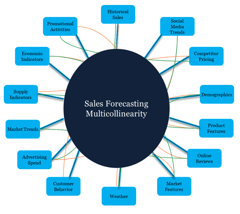
In traditional Supply Chain forecasting, algorithms typically consider a handful of variables: historical sales, seasonality, promotions, and economic indicators. Modern demand planning solutions now incorporate dozens or even hundreds of other features: real-time market sentiment, competitor pricing, weather patterns, social media trends, supply disruptions, and granular customer behavior data.
An explosion of new available data brings tremendous opportunities but also amplifies the risk of correlated features undermining forecast model reliability and interpretability. We need to understand the complex data relationships rather than treating them as a black box.
The Hidden Costs of Correlated Features
When predictor variables are highly correlated, several problems can emerge regardless of your modeling approach:
Model Instability: Small changes in training data can lead to dramatically different model predictions. This is particularly problematic in Supply Chain planning where consistency and reliability are paramount.
Misleading Feature Importance: A model might assign high importance to redundant variables while overlooking truly predictive features. This can lead to misleading business decisions concerning which factors actually drive demand.
Overfitting Risk: Highly correlated features can cause models to memorize noise rather than learn genuine patterns, resulting in poor performance with new data.
Reduced Interpretability: When multiple correlated variables contribute to predictions, it becomes nearly impossible to understand which factors truly influence demand. This can be a critical issue when explaining forecasts to stakeholders.
Detecting Variable Relationships in Modern Contexts
While statistical foundations remain relevant to modelling, modern approaches to detecting multicollinearity have evolved significantly:
Traditional Statistical Approaches (Still Valuable)
Variance Inflation Factor (VIF): Calculate VIF = 1/(1-R²) for each variable. Values above the 5-10 range indicate high multicollinearity.
Correlation Matrices: Heat maps of pairwise correlations quickly reveal obvious relationships, for example between variables like "units sold" and "retail price."
Modern Detection Methods
Recursive Feature Elimination: Systematically remove single features to evaluate the impact on model performance across validation sets.
Permutation Importance: Shuffle individual features and then measure decrease in model accuracy to identify truly important variables.
SHAP (SHapley Additive exPlanations): Provides unified measure of feature importance that accounts for feature interactions, particularly valuable for complex models.
Common Culprits in Supply Chain Data
Modern demand planning datasets often contain these multicollinearity-prone variable groups:
Time-Based Features: Week number, month, quarter, and seasonal indicators frequently correlate strongly with each other.
Economic Indicators: GDP growth, consumer confidence, and unemployment rates often move together.
Promotional Variables: Different promotion types, discount percentages, and promotional timing can create redundant signals.
Geographic Features: Regional, territory, and market-level data often exhibit strong spatial correlations.
Product Hierarchy: Category, subcategory, and brand-level variables naturally correlate within product families.
Modern Solutions for Variable Selection
Advanced Feature Selection
Regularization Methods: LASSO (L1) and Ridge (L2) regression automatically handle multicollinearity by penalizing correlated features. Elastic Net combines both approaches for optimal variable selection.
Tree-Based Feature Importance: Random Forests and Gradient Boosting Machines naturally handle correlated features and provide robust importance rankings.
Dimensionality Reduction: Principal Component Analysis (PCA) or modern alternatives like UMAP can transform correlated features into uncorrelated components while preserving predictive power.
Information Criteria for Model Comparison
The Akaike Information Criterion (AIC) remains valuable, but modern practitioners often use:
Cross-Validation Scores: More robust than single-sample AIC for assessing true model performance.
Bayesian Information Criterion (BIC): Penalizes model complexity more heavily than AIC, particularly useful for large datasets.
Business-Specific Metrics: MAPE (Mean Absolute Percentage Error) and bias metrics that directly relate to supply chain KPIs.
Machine Learning Approaches to Variable Relationships
Neural Networks and Deep Learning
While neural networks can theoretically learn to handle correlated inputs, multicollinearity still affects training stability and convergence. Techniques like dropout, batch normalization, and early stopping help, but preprocessing to reduce correlation often improves results.
Ensemble Methods
Random Forests and Gradient Boosting Machines are more robust when exposed to multicollinearity than linear models, however feature selection still improves interpretability and can enhance performance.
AutoML and Automated Feature Engineering
Modern AutoML platforms automatically detect and handle multicollinearity, but understanding feature relationships remains crucial for:
- Validating automated decisions
- Explaining model behavior to business stakeholders
- Troubleshooting unexpected model performance
Practical Implementation Framework
Phase 1: Discovery and Assessment
- Exploratory Data Analysis: Create correlation matrices and identify obvious relationships.
- Statistical Testing: Calculate VIF scores for key variables.
- Business Logic Review: Identify conceptually-related variables that might correlate well with business.
Phase 2: Intelligent Feature Selection
- Domain-Driven Grouping: Group related variables by business logic.
- Progressive Elimination: Use cross-validation to compare models with different feature sets.
- Performance Validation: Test final models on holdout data representing recent business conditions.
Phase 3: Ongoing Monitoring
- Model Drift Detection: Monitor for changing correlations as business conditions evolve.
- Feature Importance Tracking: Regularly assess whether key variables remain predictive.
- Business Alignment: Ensure model behavior continues to align with supply chain realities.
Real-World Impact: Consumer Goods Supply Chain Case Study
Consider a consumer goods company forecasting demand across ten thousand SKUs. The initial model used included more than fifty variables, including historical sales patterns, promotional activities, competitor data, economic indicators, and seasonal factors. Despite using advanced gradient boosting models, forecasting accuracy plateaued.
By systematically addressing multicollinearity, consolidating correlated promotional variables, creating composite economic indices, and removing redundant seasonal features, demand planners then reduced the feature set to twenty-five carefully selected variables. The result: 15% improvement in forecast accuracy and significantly more stable predictions across different time periods.
Looking Forward: The Future of Variable Selection
As Supply Chain data becomes increasingly complex, several modelling trends are emerging:
Automated Feature Engineering: AI systems automatically create and select optimal feature combinations while managing correlations.
Real-Time Adaptation: Models continuously adjust feature selection as market conditions change.
Causal Inference: Moving beyond correlation to understand true cause-and-effect relationships between demand drivers.
Explainable AI: Enhanced interpretation methods that help Supply Chain professionals understand complex model decisions.
Key Takeaways for Supply Chain Professionals
- Multicollinearity affects all model types, from simple regression to complex neural networks. Don't assume advanced algorithms automatically solve correlation problems.
- Feature selection is as important as model selection. A simpler model with well-chosen variables often outperforms a complex model with redundant features.
- Business understanding enhances statistical analysis. Domain expertise helps identify which correlated variables to keep and which to eliminate.
- Validation must reflect business reality. Test models on data that represent the conditions where they'll actually be used.
- Interpretability matters in supply chain planning. Stakeholders need to understand and trust the factors driving forecasts.
The fundamental challenge of managing variable relationships hasn't disappeared in the age of AI; it's become more critical than ever. By combining statistical rigor with modern Machine Learning techniques and deep supply chain expertise, we can build more accurate, stable, and interpretable demand planning models.
Ready to improve your demand forecasting accuracy? Contact Areté to learn how modern variable selection techniques can transform your planning processes.